nccsdata Part 3: Geographic Filters
Introduction
In part 3 of this 4-part series on the
nccsdata package, we
cover how to filter downloaded NCCS data based on geography.
Legacy NCCS data consists of several geographic variables, such as:
STATE: 2 letter state abbreviation (all caps)CITY: Name of the city associated with the address provided inADDRESS(all caps)FIPS: State + County FIPS codes (CBSA) as used by the US Census (five-digit integer)
The last variable, FIPS, can be used to match observations based on census units. This preserves the external validity of geographic units by aligning them with US census delineations.
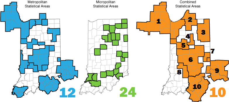
In US census data, FIPS are also tied to Core Based Statistical Areas (CBSAs) that consist of mutually exclusive Metropolitan Statistical Areas (metros with populations above 50,000) and Micropolitan Statistical Areas (populations above 10,000 and below 50,000). Geographic filtering with US census units therefore requires crosswalking units across multiple levels, such as county and CBSA.
Further details and examples of CBSAs and Metropolitan/Micropolitan Statistical Areas are provided on the Census Crosswalks page of the Urban NCCS Site.
All Census-defined metro areas are comprised of counties. This vignette
explores the process of filtering nonprofit data by geography using
geo_preview()
and
map_countyfips()
to identify the County FIPS associated with specific Metropolitan or
Micropolitan Regions.
Exploring CBSA FIPS Codes
The
geo_preview()
function allows users to preview and retrieve CBSA FIPS codes and/or
their associated metadata from a specific state.
geo_preview(
  geo    = c("cbsa","cbsafips"),
  within = "FL",
  type   = "metro" )
#>
#>
#> |                                        cbsa| cbsafips|
#> |-------------------------------------------:|--------:|
#> |                             Gainesville, FL|    23540|
#> |                            Jacksonville, FL|    27260|
#> |           Panama City-Panama City Beach, FL|    37460|
#> |           Palm Bay-Melbourne-Titusville, FL|    37340|
#> |   Miami-Fort Lauderdale-West Palm Beach, FL|    33100|
#> |                             Punta Gorda, FL|    39460|
#> |                       Homosassa Springs, FL|    26140|
#> |                     Naples-Marco Island, FL|    34940|
#> |              Pensacola-Ferry Pass-Brent, FL|    37860|
#> |      Deltona-Daytona Beach-Ormond Beach, FL|    19660|
#> |                             Tallahassee, FL|    45220|
#> |         Tampa-St. Petersburg-Clearwater, FL|    45300|
#> |                                 Sebring, FL|    42700|
#> | Sebastian-Vero Beach-West Vero Corridor, FL|    42680|
#> |               Orlando-Kissimmee-Sanford, FL|    36740|
#> |                   Cape Coral-Fort Myers, FL|    15980|
#> |           North Port-Bradenton-Sarasota, FL|    35840|
#> |                                   Ocala, FL|    36100|
#> |                          Port St. Lucie, FL|    38940|
#> |      Crestview-Fort Walton Beach-Destin, FL|    18880|
#> |                   Lakeland-Winter Haven, FL|    29460|
#> |                   Wildwood-The Villages, FL|    48680|
Specifically, filtering on geography requires using GEOIDs (the FIPS codes associated with a specific level of geo aggregation). This is because (1) city and county names are non-unique, and (2) they are long and would be easy to misspell. The geo_preview() function offers a convenient way to identify all of the GEOIDs associated with your desired geography.
The code snippet above demonstrates that
geo_preview()
returns the names of all CBSAs and their associated GEOIDs. The
within argument specifies the desired state, in abbreviated form, as
input while the geo argument returns the specified columns. The
type argument specified which type of geography is desired.
The geo argument allows uses to select a variety of columns from the geographic crosswalk file.
geo_preview(
  geo    = c("cbsa","county","cbsafips"),
  within = "FL",
  type   = "metro"  )
#>
#>
#> |                                        cbsa|                           county| cbsafips|
#> |-------------------------------------------:|--------------------------------:|--------:|
#> |                             Gainesville, FL|      Alachua County, FL, Central|    23540|
#> |                            Jacksonville, FL|       Baker County, FL, Outlying|    27260|
#> |           Panama City-Panama City Beach, FL|          Bay County, FL, Central|    37460|
#> |           Palm Bay-Melbourne-Titusville, FL|      Brevard County, FL, Central|    37340|
#> |   Miami-Fort Lauderdale-West Palm Beach, FL|      Broward County, FL, Central|    33100|
#> |                             Punta Gorda, FL|    Charlotte County, FL, Central|    39460|
#> |                       Homosassa Springs, FL|       Citrus County, FL, Central|    26140|
#> |                            Jacksonville, FL|         Clay County, FL, Central|    27260|
#> |                     Naples-Marco Island, FL|      Collier County, FL, Central|    34940|
#> |                            Jacksonville, FL|        Duval County, FL, Central|    27260|
#> |              Pensacola-Ferry Pass-Brent, FL|     Escambia County, FL, Central|    37860|
#> |      Deltona-Daytona Beach-Ormond Beach, FL|      Flagler County, FL, Central|    19660|
#> |                             Tallahassee, FL|     Gadsden County, FL, Outlying|    45220|
#> |                             Gainesville, FL|   Gilchrist County, FL, Outlying|    23540|
#> |         Tampa-St. Petersburg-Clearwater, FL|    Hernando County, FL, Outlying|    45300|
#> |                                 Sebring, FL|    Highlands County, FL, Central|    42700|
#> |         Tampa-St. Petersburg-Clearwater, FL| Hillsborough County, FL, Central|    45300|
#> | Sebastian-Vero Beach-West Vero Corridor, FL| Indian River County, FL, Central|    42680|
#> |                             Tallahassee, FL|   Jefferson County, FL, Outlying|    45220|
#> |               Orlando-Kissimmee-Sanford, FL|        Lake County, FL, Outlying|    36740|
#> |                   Cape Coral-Fort Myers, FL|          Lee County, FL, Central|    15980|
#> |                             Tallahassee, FL|         Leon County, FL, Central|    45220|
#> |                             Gainesville, FL|        Levy County, FL, Outlying|    23540|
#> |           North Port-Bradenton-Sarasota, FL|      Manatee County, FL, Central|    35840|
#> |                                   Ocala, FL|       Marion County, FL, Central|    36100|
#> |                          Port St. Lucie, FL|       Martin County, FL, Central|    38940|
#> |   Miami-Fort Lauderdale-West Palm Beach, FL|   Miami-Dade County, FL, Central|    33100|
#> |                            Jacksonville, FL|      Nassau County, FL, Outlying|    27260|
#> |      Crestview-Fort Walton Beach-Destin, FL|     Okaloosa County, FL, Central|    18880|
#> |               Orlando-Kissimmee-Sanford, FL|       Orange County, FL, Central|    36740|
#> |               Orlando-Kissimmee-Sanford, FL|     Osceola County, FL, Outlying|    36740|
#> |   Miami-Fort Lauderdale-West Palm Beach, FL|   Palm Beach County, FL, Central|    33100|
#> |         Tampa-St. Petersburg-Clearwater, FL|        Pasco County, FL, Central|    45300|
#> |         Tampa-St. Petersburg-Clearwater, FL|     Pinellas County, FL, Central|    45300|
#> |                   Lakeland-Winter Haven, FL|         Polk County, FL, Central|    29460|
#> |                            Jacksonville, FL|    St. Johns County, FL, Central|    27260|
#> |                          Port St. Lucie, FL|    St. Lucie County, FL, Central|    38940|
#> |              Pensacola-Ferry Pass-Brent, FL|   Santa Rosa County, FL, Central|    37860|
#> |           North Port-Bradenton-Sarasota, FL|     Sarasota County, FL, Central|    35840|
#> |               Orlando-Kissimmee-Sanford, FL|     Seminole County, FL, Central|    36740|
#> |                   Wildwood-The Villages, FL|       Sumter County, FL, Central|    48680|
#> |      Deltona-Daytona Beach-Ormond Beach, FL|      Volusia County, FL, Central|    19660|
#> |                             Tallahassee, FL|     Wakulla County, FL, Outlying|    45220|
#> |      Crestview-Fort Walton Beach-Destin, FL|       Walton County, FL, Central|    18880|
#> |           Panama City-Panama City Beach, FL|  Washington County, FL, Outlying|    37460|
Metropolitan and Micropolitan Data
Because CBSAs include combinations of metropolitan or micropolitan
statistical
areas,
geo_preview()
allows the user to select either unit using the type argument.
The following code snippet shows how to retrieve CBSA names and FIPS codes for all metropolitan statistical areas in Wyoming:
geo_preview(
  geo    = c("cbsa","cbsafips"),
  within = "WY",
  type   = "metro" )
#>
#>
#> |         cbsa| cbsafips|
#> |------------:|--------:|
#> | Cheyenne, WY|    16940|
#> |   Casper, WY|    16220|
In the above snippet, setting type to micro returns data for micropolitan statistical areas.
geo_preview(
  geo    = c("cbsa","cbsafips"),
  within = "WY",
  type   = "micro" )
#>
#>
#> |             cbsa| cbsafips|
#> |----------------:|--------:|
#> |      Laramie, WY|    29660|
#> |     Gillette, WY|    23940|
#> |     Riverton, WY|    40180|
#> |         Cody, WY|    17650|
#> |     Sheridan, WY|    43260|
#> | Rock Springs, WY|    40540|
#> |   Jackson, WY-ID|    27220|
#> |  Evanston, WY-UT|    21740|
Exploring CSA FIPS
Core Based Statistical Areas (CBSAs) delineate the distinct metropolitan areas. The Combined Statistical Areas (CSA) geography aggregates the data further into metropolital regions where multiple cities function as a coherent entities, typically characterized by shared commercial and commuting zones.
Similar to how metro areas area comprised of a collection of counties, you can think of the Combined Statistical Areas as being comprised of collections of metropolitan and micropolitan areas.
939 Core-Based Statistical Areas =
    384 Metropolitan statistical areas +
    547 micropolitan statistical areas

175 Total Combined Statistical Areas:
    808 Metro + Micro Areas joined together to form CSAs
    123 Metro + Micro Areas are not part of any CSA
geo_preview()
can retrieve metadata for Combined Statistical
Areas (CSAs).
The code snippet below returns all CSA names and FIPS codes for metropolitan statistical areas in Virginia:
geo_preview(
  geo    = c("csa","csafips"),
  within = "VA",
  type   = "metro")
#>
#>
#> |                                            csa| csafips|
#> |----------------------------------------------:|-------:|
#> |                                               |      NA|
#> | Washington-Baltimore-Arlington, DC-MD-VA-WV-PA|     548|
#> |        Harrisonburg-Staunton-Stuarts Draft, VA|     277|
#> |               Virginia Beach-Chesapeake, VA-NC|     545|
#> |          Johnson City-Kingsport-Bristol, TN-VA|     304|
Filtering Legacy Data with County FIPS codes
After retrieving the desired CBSA/CSA FIPS codes,
map_countyfips()
can match them with county FIPS codes present in the legacy data,
retrieved with
get_data().
Downloaded data can then be filtered using these county FIPS codes, as
shown below:
# Retrive CBSA FIPS from NY
cbsa_ny <-
  geo_preview( geo = c("cbsa", "cbsafips"),
               within = "NY" )
#>
#>
#> |                                  cbsa| cbsafips|
#> |-------------------------------------:|--------:|
#> |           Albany-Schenectady-Troy, NY|    10580|
#> |    New York-Newark-Jersey City, NY-NJ|    35620|
#> |                        Binghamton, NY|    13780|
#> |                             Olean, NY|    36460|
#> |                            Auburn, NY|    12180|
#> |                 Jamestown-Dunkirk, NY|    27460|
#> |                            Elmira, NY|    21300|
#> |                       Plattsburgh, NY|    38460|
#> |                            Hudson, NY|    26460|
#> |                          Cortland, NY|    18660|
#> | Kiryas Joel-Poughkeepsie-Newburgh, NY|    28880|
#> |               Buffalo-Cheektowaga, NY|    15380|
#> |                      Gloversville, NY|    24100|
#> |                           Batavia, NY|    12860|
#> |                        Utica-Rome, NY|    46540|
#> |               Watertown-Fort Drum, NY|    48060|
#> |                         Rochester, NY|    40380|
#> |                          Syracuse, NY|    45060|
#> |                         Amsterdam, NY|    11220|
#> |                           Oneonta, NY|    36580|
#> |                Massena-Ogdensburg, NY|    32390|
#> |                      Seneca Falls, NY|    42900|
#> |                           Corning, NY|    18500|
#> |                        Monticello, NY|    33910|
#> |                            Ithaca, NY|    27060|
#> |                          Kingston, NY|    28740|
#> |                       Glens Falls, NY|    24020|

# Map these to county FIPS codes
ny_countyfips <-
  map_countyfips( geo.cbsafips = cbsa_ny$cbsafips )

# Pull core data for the year 2015
core_2015 <-
  get_data( dsname         = "core",
            time           = "2015",
            scope.orgtype  = "NONPROFIT",
            scope.formtype = "PZ" )
#> Valid inputs detected. Retrieving data.
#> Downloading core data
#> Requested files have a total size of 115 MB. Proceed
#>                       with download? Enter Y/N (Yes/no/cancel)
#> Core data downloaded

# Filter with NY county FIPS
core_2015_nyfips <-
  core_2015 %>%
  dplyr::filter( FIPS %in% ny_countyfips )

print( as_tibble( core_2015_nyfips ))
#> # A tibble: 11,788 × 170
#>    NTEECC new.code   type.org broad.category major.group univ  hosp  two.digit
#>    <chr>  <chr>      <chr>    <chr>          <chr>       <lgl> <lgl> <chr>
#>  1 N50    RG-HMS-N50 RG       HMS            N           FALSE FALSE 50
#>  2 Y42    RG-MMB-Y42 RG       MMB            Y           FALSE FALSE 42
#>  3 P012   <NA>       <NA>     <NA>           <NA>        NA    NA    <NA>
#>  4 S47    RG-PSB-S47 RG       PSB            S           FALSE FALSE 47
#>  5 N50    RG-HMS-N50 RG       HMS            N           FALSE FALSE 50
#>  6 S41    RG-PSB-S41 RG       PSB            S           FALSE FALSE 41
#>  7 J40    RG-HMS-J40 RG       HMS            J           FALSE FALSE 40
#>  8 J40    RG-HMS-J40 RG       HMS            J           FALSE FALSE 40
#>  9 B41    RG-UNI-B41 RG       UNI            B           TRUE  FALSE 41
#> 10 M24    RG-HMS-M24 RG       HMS            M           FALSE FALSE 24
#> # ℹ 11,778 more rows
#> # ℹ 162 more variables: further.category <int>, division.subdivision <chr>,
#> #   broad.category.description <chr>, major.group.description <chr>,
#> #   code.name <chr>, division.subdivision.description <chr>, keywords <chr>,
#> #   further.category.desciption <chr>, ntee2.code <chr>, EIN <int>,
#> #   ACCPER <chr>, ACTIV1 <chr>, ACTIV2 <chr>, ACTIV3 <chr>, ADDRESS <chr>,
#> #   AFCD <chr>, ASS_BOY <dbl>, ASS_EOY <int64>, BLOCK <chr>, BOND_BOY <dbl>, …
Conclusion
Using FIPS codes allows researchers working with NCCS data to standardize their operationalized geographic variables, resulting in greater external validity and reproducibility in their research.
nccsdata Part 4: Summary Tables
Part 4 of 4 data stories covering the nccsdata R package. This story focuses on summarising NCCS legacy data.
nccsdata Part 2: NTEE Codes
Part 2 of 4 data stories covering the nccsdata R package. This story focuses on parsing NTEE codes.